Metrics Used to Compare Histograms

Introduction

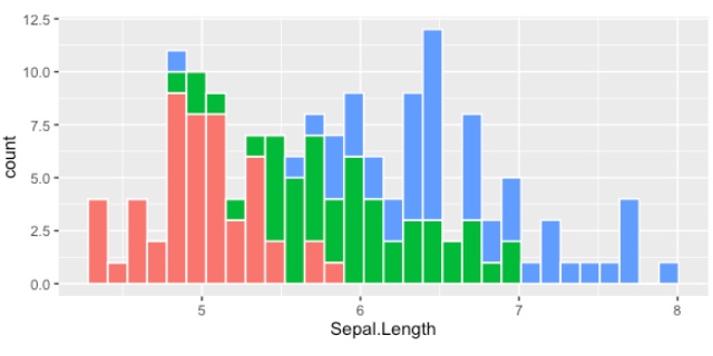
Comparing histograms is a crucial step in data analysis, as it allows us to gain insights into the underlying distributions of our data. There are several metrics that can be used to compare histograms, each with its own strengths and weaknesses. In this article, we will discuss some of the most commonly used metrics for comparing histograms and provide examples of how to calculate them in Python.

• Most common methods
  • 1. Chi-Squared Distance
  • 2. Earth Mover's Distance
  • 3. Kullback-Leibler Divergence
• Other methods for histogram comparison
• Conclusion

Most common methods

1. Chi-Squared Distance

The Chi-Squared distance, also known as the Chi-Squared test, measures the difference between two histograms by comparing the observed frequencies to the expected frequencies. The Chi-Squared distance is defined as:

Where \(O_i\) is the observed frequency in bin \(i\), \(E_i\) is the expected frequency in bin \(i\), and \(n\) is the number of bins. The Chi-Squared distance is sensitive to large differences between the observed and expected frequencies, and is commonly used in hypothesis testing to determine if two histograms come from the same distribution.

To calculate the Chi-Squared distance in Python, we can use the scipy.stats.chisquare function from the SciPy library. Here is an example of how to use this function to calculate the Chi-Squared distance between two histograms:

from scipy.stats import chisquare

# observed frequencies
obs1 = [10, 20, 30, 40]
obs2 = [15, 25, 35, 45]

# calculate the Chi-Squared distance
chi2, p = chisquare(obs1, obs2)

print(chi2)

2. Earth Mover's Distance

The Earth Mover's distance (EMD) is a more sophisticated metric that takes into account the shape of the histograms as well as the differences in frequency. The EMD is defined as the minimum amount of "work" required to transform one histogram into the other, where "work" is defined as the product of the difference in frequency and the distance between the bins. The EMD is commonly used in image processing and computer vision, but can also be used to compare histograms.

To calculate the EMD in Python, we can use the emd function from the pyemd library. Here is an example of how to use this function to calculate the EMD between two histograms:

import numpy as np
from pyemd import emd

# histogram bin centers
bins1 = [1, 2, 3, 4]
bins2 = [1.5, 2.5, 3.5, 4.5]

# histogram frequencies
freq1 = [10, 20, 30, 40]
freq2 = [15, 25, 35, 45]

# calculate the EMD
emd_val = emd(bins1, bins2, freq1, freq2)

print(emd_val)

3. Kullback-Leibler Divergence

The Kullback-Leibler divergence (KLD), also known as the relative entropy, measures the difference between two probability distributions. The KLD is defined as:

Where \(P\) is the probability distribution of the first histogram, \(Q\) is the probability distribution of the second histogram, and \(n\) is the number of bins. The KLD is a measure of the information lost when approximating one histogram with the other. It is commonly used in information theory and machine learning.

To calculate the KLD in Python, we can use the scipy.stats.entropy function from the SciPy library. Here is an example of how to use this function to calculate the KLD between two histograms:

from scipy.stats import entropy

# histogram frequencies
freq1 = [10, 20, 30, 40]
freq2 = [15, 25, 35, 45]

# normalize the frequencies to get probability distributions
prob1 = freq1 / np.sum(freq1)
prob2 = freq2 / np.sum(freq2)

# calculate the KLD
kld = entropy(prob1, prob2)

print(kld)

Other methods for histogram comparison

• Intersection: it is a simple but widely used measure, which counts the number of bins where the histograms overlap. This metric gives a value between 0 and the minimum number of samples in the two histograms, with 0 indicating no overlap and the maximum value indicating perfect overlap.

• Bhattacharyya Distance: The Bhattacharyya distance is a measure of similarity between two histograms. It is based on the Bhattacharyya coefficient, which is a measure of the similarity of two probability distributions.

• Wasserstein Distance: Also known as the "Earth Mover's Distance" (EMD), it is a distance measure between probability distributions. It is widely used in image processing and computer vision, and has been applied to the comparison of histograms.

There are other metrics such as Hellinger distance, Jeffreys divergence, Jensen-Shannon divergence, etc. that can be used to compare histograms as well.

Conclusion

There are several metrics that can be used to compare histograms, each with its own strengths and weaknesses.

• The Chi-Squared distance is sensitive to large differences in frequency,
• the Earth Mover's Distance takes into account the shape of the histograms, and
• the Kullback-Leibler Divergence measures the information lost when approximating one histogram with the other.

By understanding these metrics and how to calculate them in Python, data scientists can choose the most appropriate metric for their analysis and gain deeper insights into the underlying distributions of their data.

It is always recommended to try out different metrics and choose the best one that suits the problem and data.

To learn more about these metrics and other techniques for comparing histograms, visit the following resources:

• Chi-Squared Test
• Earth Mover's Distance
• Kullback-Leibler Divergence
• pyemd library
• SciPy library